Plotting Benchmark Results with matplotlib
The Zig and Go posts about sharded locks have the same kind of plots: a scaling plot, a bar chart with a group per workload, a shard count curve and in the Go post a fourth one with more goroutines than cores. Both posts say that a shell loop and a short Python script made them and leave it there. This post is the loop and the script. I reran both benchmarks while writing it, so the plots below come from fresh data and the numbers differ a little from the ones in the other two posts.
The raw data Link to heading
The two benchmark programs take the same four arguments: the lock type, the number of shards, the read percentage and the number of threads or goroutines. Both print one line of CSV with the nanoseconds per operation at the end:
mutex,64,50,8,19.1
There is one difference between them. The Zig program prints its line with std.debug.print(), which writes to standard error. The Go program prints with fmt.Printf(), which writes to standard output. The loop redirects both streams into the file, so it does not care which one the program used. If you only redirect standard output you get an empty CSV file from the Zig program and no error message. The other way round, when a run fails its error output lands in the CSV file as well and the script stops at the first line it cannot read, so look at the file before you plot it.
The loop Link to heading
The loop runs every combination 5 times and prints the lines as they come, so you redirect its output into a file and that file is your raw data. Every plot in this post can be made again from it and when a number looks odd you can look at the five runs behind it.
#!/bin/sh
# Runs every combination of the benchmark 5 times and prints one CSV line per run.
# Usage: ./bench.sh ./locks > zig.csv
#        ./bench.sh ./locks go > go.csv   (adds the goroutine sweep)
bin=$1
runs=5

for i in $(seq $runs); do
    for lock in mutex rwlock; do
        for shards in 1 64; do
            for reads in 100 90 50 10; do
                for threads in 1 2 4 8; do
                    $bin $lock $shards $reads $threads 2>&1
                done
            done
        done
    done
    for shards in 4 16 256 1024; do
        $bin mutex $shards 50 8 2>&1
    done
    if [ "$2" = go ]; then
        for lock in mutex rwlock; do
            for shards in 1 64; do
                for goroutines in 16 32 64 256 1024; do
                    $bin $lock $shards 50 $goroutines 8 2>&1
                done
            done
        done
    fi
done
The outer loop is over the passes and the inner loops are over the parameters, so each pass runs every combination once before any combination runs twice. If the machine does something else for a minute, that minute hits one run of many combinations instead of all five runs of one combination and the median throws it away. The shard sweep only needs the counts that the main loops do not cover, which is why it runs 4, 16, 256 and 1024 and not 1 and 64. The goroutine sweep passes 8 as a fifth argument that the Go program uses for GOMAXPROCS and it only runs when you say go, because the Zig program stops at 64 threads.
This is how I ran it, with each program built in its own directory:
$ ./bench.sh ./zig/locks > zig.csv
$ ./bench.sh ./go/locks go > go.csv
$ wc -l zig.csv go.csv
     340 zig.csv
     440 go.csv
The Zig loop took about 4 minutes and the Go loop about 10, because every Go run is slower and the goroutine sweep adds 100 runs, half of them with a single contended lock.
The script Link to heading
The script reads the CSV file, takes the median of every group of runs and draws the plots. It needs matplotlib and nothing else, because the Standard Library of Python has a CSV reader and a median() function and that is all the data processing there is. It selects the Agg backend before it imports pyplot and writes every plot with savefig(), so it never opens a window and runs the same on a server without a display and in a shell loop of its own.
import csv
import math
import sys
from collections import defaultdict
from statistics import median

import matplotlib
matplotlib.use("Agg")
import matplotlib.pyplot as plt
from matplotlib.ticker import FixedLocator, NullLocator, FuncFormatter

# Usage: python3 plots.py results.csv threads
# The second argument is the word for the x axis, threads or goroutines.
csv_path = sys.argv[1]
unit = sys.argv[2] if len(sys.argv) > 2 else "threads"

# The name of each design comes from the lock type and the shard count.
names = {("mutex", 1): "mutex", ("rwlock", 1): "rwlock",
         ("mutex", 64): "sharded", ("rwlock", 64): "sharded-rw"}
colors = {"mutex": "#2b7bde", "rwlock": "#f0603c",
          "sharded": "#1fb27a", "sharded-rw": "#f0a500"}
designs = ["mutex", "rwlock", "sharded", "sharded-rw"]
workloads = [(100, "read-only"), (90, "read-heavy\n90% reads"),
             (50, "balanced\n50% reads"), (10, "write-heavy\n10% reads")]

# Group the runs by their four parameters and keep the median.
runs = defaultdict(list)
with open(csv_path) as f:
    for lock, shards, reads, threads, value in csv.reader(f):
        runs[(lock, int(shards), int(reads), int(threads))].append(float(value))
ns = {k: median(v) for k, v in runs.items()}

def lookup(design, reads, threads):
    lock, shards = next(k for k, v in names.items() if v == design)
    return ns.get((lock, shards, reads, threads))

def figure(height=4.6):
    fig, ax = plt.subplots(figsize=(7.5, height), dpi=150)
    fig.patch.set_facecolor("#fafafa")
    ax.set_facecolor("#fafafa")
    ax.grid(True, color="#e3e3e3", linewidth=0.8, zorder=0)
    for s in ax.spines.values():
        s.set_color("#dddddd")
    ax.tick_params(colors="#555", labelsize=11, length=0)
    return fig, ax

def log_axis(ax, ticks):
    ax.set_yscale("log")
    ax.yaxis.set_major_locator(FixedLocator(ticks))
    ax.yaxis.set_minor_locator(NullLocator())
    ax.yaxis.set_major_formatter(FuncFormatter(lambda v, _: f"{int(v)}"))
    ax.set_ylabel("ns per operation (log scale)", fontsize=12, color="#444")

def spread(ends, gap, log=False):
    # Push the end labels apart when two lines finish too close to each other.
    # On a log axis the gap is a ratio, so the work happens on the logarithms.
    order = sorted(ends, key=ends.get)
    ys = [math.log10(ends[d]) if log else ends[d] for d in order]
    for i in range(1, len(ys)):
        if ys[i] - ys[i - 1] < gap:
            ys[i] = ys[i - 1] + gap
    return dict(zip(order, [10 ** y if log else y for y in ys]))

def save(fig, ax, title, name):
    ax.set_title(title, loc="left", fontsize=13, color="#222", pad=12)
    fig.tight_layout()
    fig.savefig(name, facecolor=fig.get_facecolor())
    print("wrote", name)

# Plot 1: speedup over one thread on the balanced workload.
threads = [1, 2, 4, 8]
fig, ax = figure()
ax.plot(threads, threads, "--", color="#555", linewidth=1.2, label="ideal")
ax.text(8.2, 8, "ideal", fontsize=11, color="#555", va="center")
ends = {}
for d in designs:
    base = lookup(d, 50, 1)
    speedup = [base / lookup(d, 50, t) for t in threads]
    ax.plot(threads, speedup, color=colors[d], linewidth=2.5, marker="o", markersize=7, label=d)
    ends[d] = speedup[-1]
for d, y in spread(ends, 0.35).items():
    ax.text(8.2, y, d, fontsize=11, color="#222", va="center")
ax.set_xticks(threads)
ax.set_xlim(0.7, 9.5)
ax.set_xlabel(unit, fontsize=12, color="#444")
ax.set_ylabel(f"speedup over 1 {unit[:-1]}", fontsize=12, color="#444")
ax.legend(loc="upper left", frameon=False, fontsize=11)
save(fig, ax, "Scaling on the balanced workload (50% reads)", "scaling.png")

# Plot 2: cost per operation with 8 threads for every workload.
fig, ax = figure()
width = 0.2
for i, d in enumerate(designs):
    xs = [j + (i - 1.5) * width for j in range(len(workloads))]
    ys = [lookup(d, reads, 8) for reads, _ in workloads]
    ax.bar(xs, ys, width=width * 0.92, color=colors[d], label=d, zorder=3)
    for x, y in zip(xs, ys):
        ax.text(x, y * 1.08, f"{y:.0f}", ha="center", fontsize=9.5, color="#222")
log_axis(ax, [10, 100, 1000])
ax.set_ylim(5, 1000)
ax.set_xticks(range(len(workloads)))
ax.set_xticklabels([w for _, w in workloads])
ax.legend(loc="upper left", ncol=4, frameon=False, fontsize=11)
save(fig, ax, f"Cost per operation with 8 {unit}", "workloads.png")

# Plot 3: the number of shards on the balanced workload with 8 threads.
shard_counts = [1, 4, 16, 64, 256, 1024]
fig, ax = figure(4.2)
ys = [ns[("mutex", s, 50, 8)] for s in shard_counts]
ax.plot(range(len(shard_counts)), ys, color=colors["sharded"], linewidth=2.5, marker="o", markersize=8, zorder=3)
for x, y in enumerate(ys):
    ax.annotate(f"{y:.0f}", (x, y), textcoords="offset points", xytext=(0, 9), ha="center", fontsize=10, color="#222")
log_axis(ax, [10, 20, 50, 100, 200, 500])
ax.set_ylim(min(ys) * 0.7, max(ys) * 1.8)
ax.set_xticks(range(len(shard_counts)))
ax.set_xticklabels([str(s) for s in shard_counts])
ax.set_xlim(-0.3, len(shard_counts) - 0.7)
ax.set_xlabel("shards", fontsize=12, color="#444")
save(fig, ax, f"Shard count, balanced workload, 8 {unit}", "shards.png")

# Plot 4: more goroutines than cores. Only drawn when the CSV has the sweep.
counts = [8, 16, 32, 64, 256, 1024]
if all(lookup("mutex", 50, c) for c in counts):
    fig, ax = figure()
    ends = {}
    for d in designs:
        ys = [lookup(d, 50, c) for c in counts]
        ax.plot(range(len(counts)), ys, color=colors[d], linewidth=2.5, marker="o", markersize=7, label=d, zorder=3)
        ends[d] = ys[-1]
    for d, y in spread(ends, 0.08, log=True).items():
        ax.text(len(counts) - 0.8, y, d, fontsize=11, color="#222", va="center")
    log_axis(ax, [10, 20, 50, 100, 200, 500])
    ax.set_ylim(9, 900)
    ax.set_xticks(range(len(counts)))
    ax.set_xticklabels([str(c) for c in counts])
    ax.set_xlim(-0.3, len(counts) + 0.3)
    ax.set_xlabel(f"{unit} on 8 cores", fontsize=12, color="#444")
    ax.legend(loc="lower left", ncol=4, frameon=False, fontsize=11)
    save(fig, ax, f"More {unit} than cores, balanced workload", "goroutines.png")
The script starts by giving the four designs their names. The CSV lines say mutex with 64 shards and the posts say sharded, so the names dictionary maps the lock type and the shard count to the name and lookup() goes the other way when a plot asks for a design by name. The colors dictionary gives every design one color that it keeps in every plot. The mutex is blue in the scaling plot, blue in the bar chart and blue in the goroutine plot, so once you have read one plot you can read the others without looking at the legend.
The runs dictionary collects the measurements under a key made of the four parameters and ns keeps the median of each group. A median of 5 runs is a good choice for benchmarks because one slow run, which happens, barely moves it, while a mean would move by a fifth of the outlier.
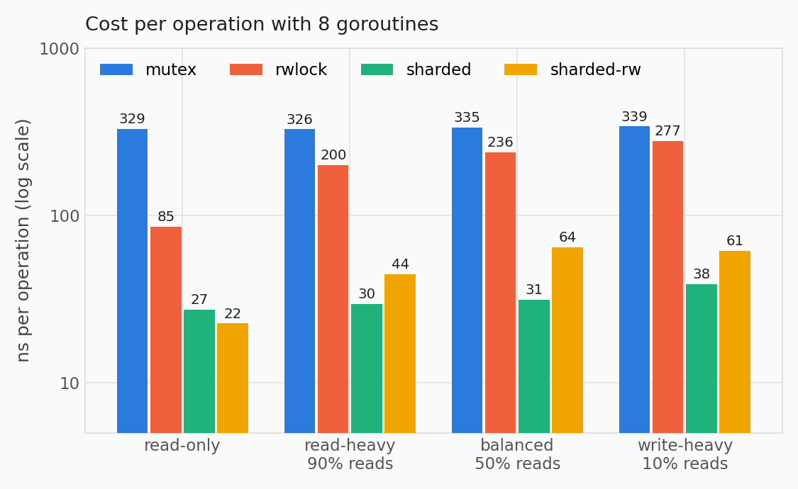
The figure() and log_axis() functions hold the style, so that the four plots look like they belong to the same post. The background is off-white, the grid is light grey, the spines are almost invisible and the ticks have no marks. The log_axis() function does something that matplotlib does not do by itself. A logarithmic axis gets labels only at the powers of ten, written as 10¹, 10² and 10³ and the minor ticks between them carry no label at all, so a reader has to guess where 50 ns or 200 ns is when the interesting range is 22 ns to 339 ns. The function places the ticks by hand with FixedLocator, removes the minor ticks with NullLocator and formats the labels as plain integers with FuncFormatter.
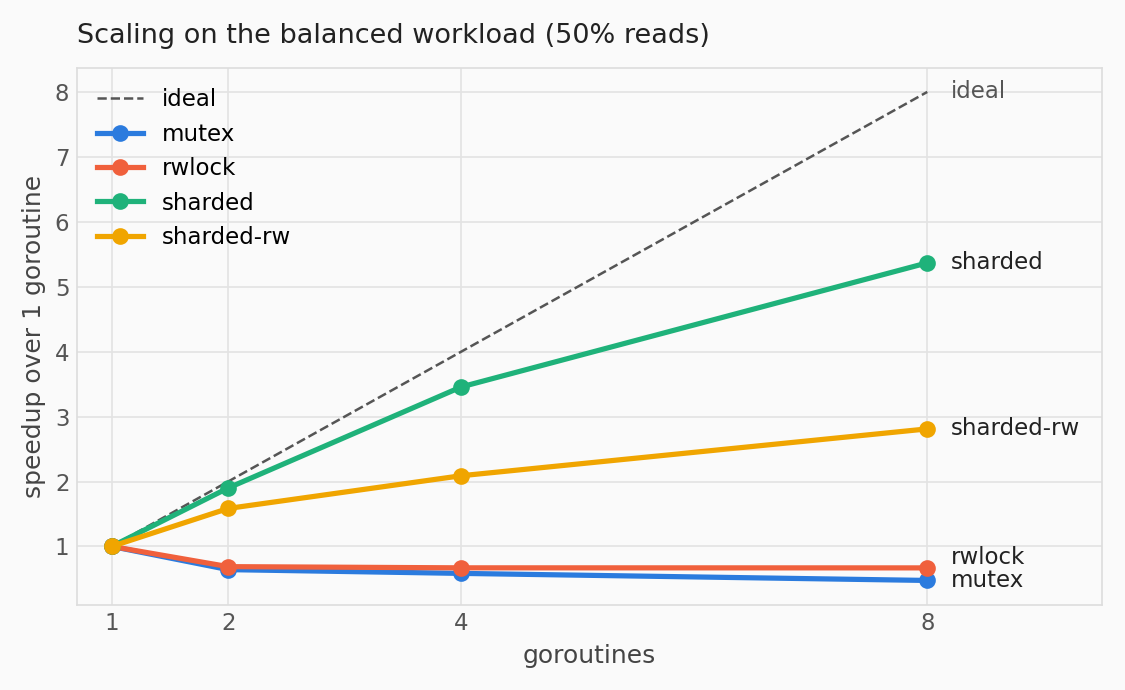
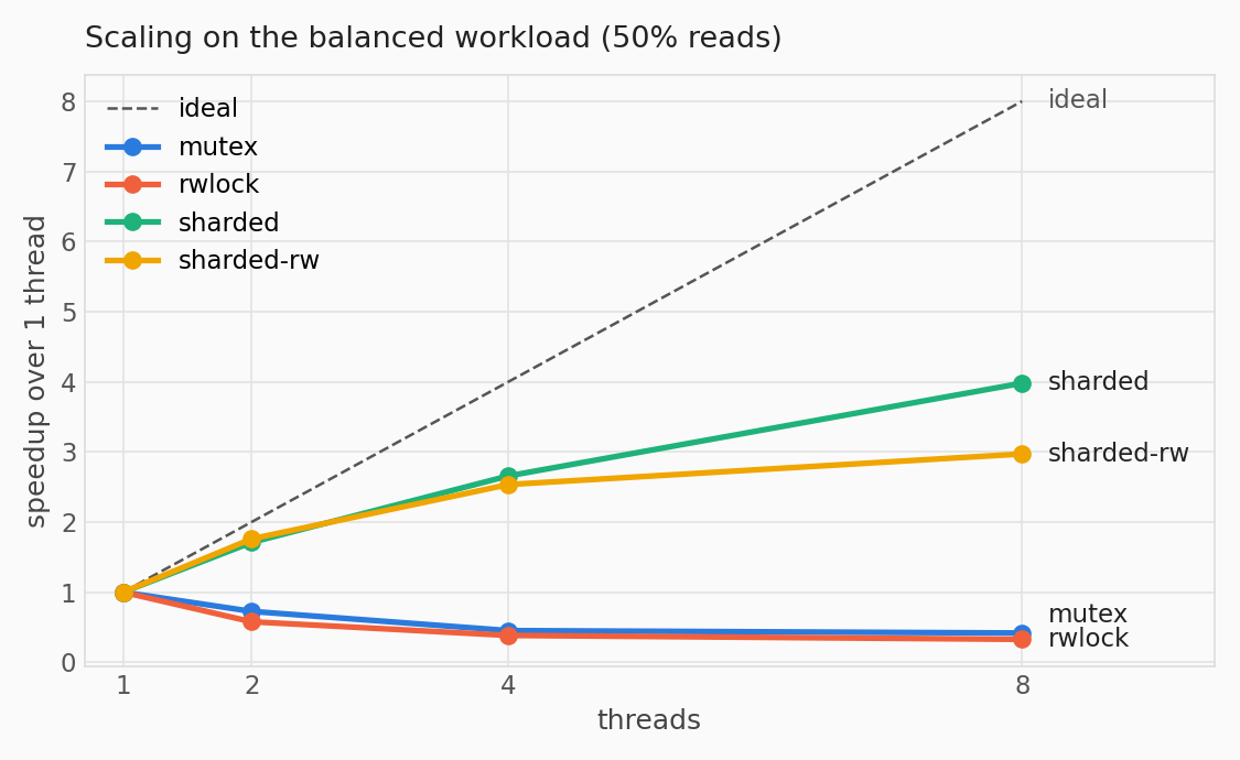
The scaling plot divides every measurement by the one thread measurement of the same design, so the y axis is a speedup and all four lines start at 1. The dashed line is the ideal and shows how far from it every design is. The labels at the right end of the lines repeat the legend, because at 8 threads the eye is at the right end of the plot and not at the legend in the top left corner. The spread() function pushes two labels apart when two lines end at almost the same value, which the mutex and the read-write lock do.
The bar chart uses a logarithmic axis because the slowest design is more than ten times slower than the fastest one and on a linear axis the sharded bars would be flat. Every bar carries its value, so the plot is also a table and nobody has to estimate a height on a log scale. The four bars of one workload sit side by side and the 0.92 factor puts a hairline between them. The gap between the groups is the fifth of the unit that four bars of width 0.2 do not fill.
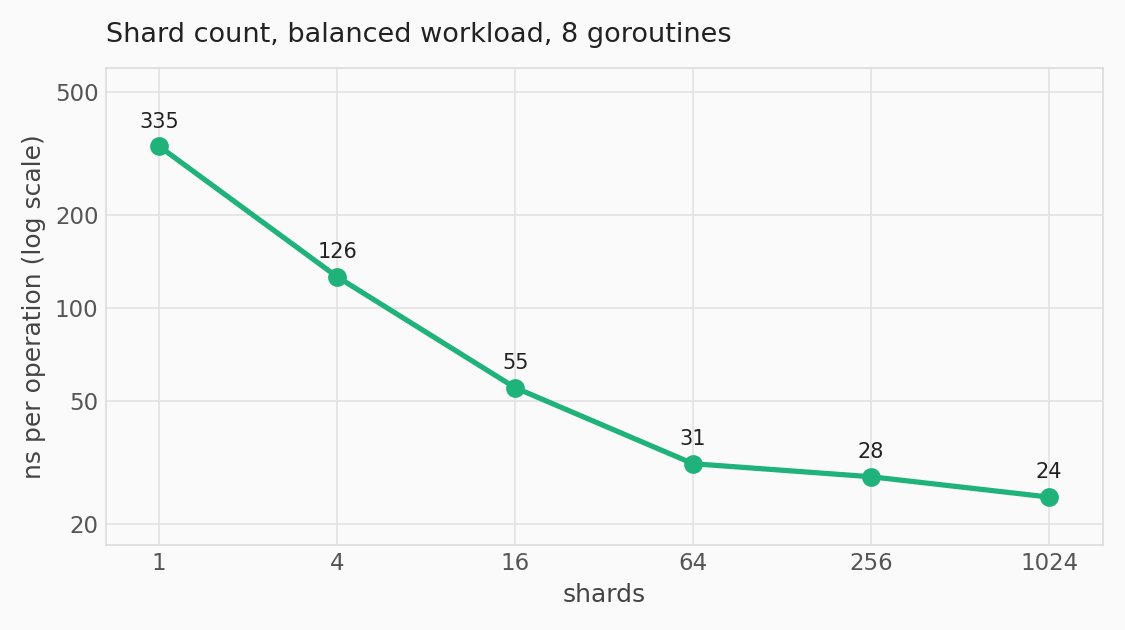
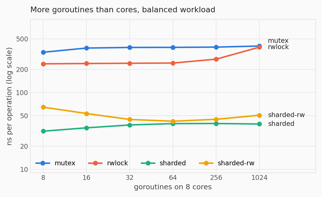
The shard count plot is the simplest one, a single line with the value next to every point. The goroutine plot only appears when the CSV file has the sweep, which the script checks with all() before it draws it.
The plots Link to heading
The script takes two arguments. The first one is the CSV file that the shell loop produced and the second one is the word for the x axis, threads or goroutines, which also goes into the titles. The second argument is optional and defaults to threads. This is the run for the Go CSV file and the four plots it made follow:
$ python3 plots.py go.csv goroutines
wrote scaling.png
wrote workloads.png
wrote shards.png
wrote goroutines.png
The same command with zig.csv and threads makes the three Zig plots. Here is the Zig scaling plot from the same session, which still says what the Zig post says:
Happy plotting!